Note
Download this example as a Jupyter notebook here: pypsa/atlite
Historic comparison PV and wind#
In this example we are examining the power feed-ins calculated by atlite. Based on data for capacity distributions and weather during the year 2013 in Germany, we try to match historical statistics.
[1]:
from collections import OrderedDict

import pandas as pd
import pgeocode
import xarray as xr

import atlite
[2]:
import matplotlib.pyplot as plt

%matplotlib inline

import seaborn as sns

sns.set_style("whitegrid")
Download Necessary Data Files#
We need to download the locations of all the PV installations in Germany to later tell atlite where to setup the PV panels and with which capacity. This information is available in Germany (thanks to the EEG feed-in-tariffs in the so-called “Anlagenregister”).
We also download a reference time-series to compare our results against later. We retrieve the data from https://open-power-system-data.org which in return gets it from ENTSO-E.
Finally we also download a cutout of weather data from the ERA5 dataset containing Germany and the year we want to examine (2012).
[3]:
import zipfile
from pathlib import Path

import requests


def download_file(url, local_filename):
    # variant of http://stackoverflow.com/a/16696317
    if not Path(local_filename).exists():
        r = requests.get(url, stream=True)
        with Path(local_filename).open("wb") as f:
            for chunk in r.iter_content(chunk_size=1024):
                if chunk:
                    f.write(chunk)
    return local_filename
Reference time-series#
The reference is downloaded from Open Power System Data (OPSD) and contains data reported by the TSOs and DSOs.
[4]:
opsd_fn = download_file(
    "https://data.open-power-system-data.org/index.php?package=time_series&version=2019-06-05&action=customDownload&resource=3&filter%5B_contentfilter_cet_cest_timestamp%5D%5Bfrom%5D=2012-01-01&filter%5B_contentfilter_cet_cest_timestamp%5D%5Bto%5D=2013-05-01&filter%5BRegion%5D%5B%5D=DE&filter%5BVariable%5D%5B%5D=solar_generation_actual&filter%5BVariable%5D%5B%5D=wind_generation_actual&downloadCSV=Download+CSV",
    "time_series_60min_singleindex_filtered.csv",
)
[5]:
opsd = pd.read_csv(opsd_fn, parse_dates=True, index_col=0)

# we later use the (in current version) timezone unaware datetime64
# to work together with this format, we have to remove the timezone
# timezone information. We are working with UTC everywhere.

opsd.index = opsd.index.tz_convert(None)

# We are only interested in the 2012 data
opsd = opsd[(opsd.index > "2011") & (opsd.index < "2013")]
PV locations (“Anlagenregister”)#
Download and unzip the archive containing all reported PV installations in Germany in 2011 from energymap.info.
[6]:
eeg_fn = download_file(
    "http://www.energymap.info/download/eeg_anlagenregister_2015.08.utf8.csv.zip",
    "eeg_anlagenregister_2015.08.utf8.csv.zip",
)

with zipfile.ZipFile(eeg_fn, "r") as zip_ref:
    zip_ref.extract("eeg_anlagenregister_2015.08.utf8.csv")
Create a Cutout from ERA5#
Load the country shape for Germany and determine its geographic bounds for downloading the appropriate cutout from ECMWF’s ERA5 data set.
[7]:
import cartopy.io.shapereader as shpreader
import geopandas as gpd

shp = shpreader.Reader(
    shpreader.natural_earth(
        resolution="10m", category="cultural", name="admin_0_countries"
    )
)
de_record = list(filter(lambda c: c.attributes["ISO_A2"] == "DE", shp.records()))[0]
de = pd.Series({**de_record.attributes, "geometry": de_record.geometry})
x1, y1, x2, y2 = de["geometry"].bounds
[8]:
cutout = atlite.Cutout(
    "germany-2012",
    module="era5",
    x=slice(x1 - 0.2, x2 + 0.2),
    y=slice(y1 - 0.2, y2 + 0.2),
    chunks={"time": 100},
    time="2012",
)
/home/fabian/vres/py/atlite/atlite/cutout.py:186: UserWarning: Arguments module, x, y, time are ignored, since cutout is already built.
  warn(
[9]:
cutout.prepare()
[9]:
<Cutout "germany-2012">
 x = 5.75 ⟷ 15.00, dx = 0.25
 y = 47.25 ⟷ 55.25, dy = 0.25
 time = 2012-01-01 ⟷ 2012-12-31, dt = H
 module = era5
 prepared_features = ['height', 'wind', 'influx', 'temperature', 'runoff']
Downloading the cutout can take a few seconds or even an hour, depending on your internet connection and whether the dataset was recently requested from the data set provider (and is thus cached on their premise). For us this took ~2 minutes the first time. Preparing it again (a second time) is snappy (for whatever reason you would want to download the same cutout twice).
Generate capacity layout#
The capacity layout represents the installed generation capacities in MW in each of the cutout’s grid cells. For this example we have generation capacities in kW on a postal code (and partially even more detailed) level. Using the following function, we load the data, fill in geocoordinates where missing for all capacities.
Below, the resulting capacities are dissolved to the grid raster using the function Cutout.layout_from_capacity_list. The dissolving is done by aggregating the capacities to their respective closest grid cell center obtained from the cutout.grid.
[10]:
def load_capacities(typ, cap_range=None, until=None):
    """
    Read in and select capacities.

    Parameters
    ----------
    typ : str
        Type of energy source, e.g. "Solarstrom" (PV), "Windenergie" (wind).
    cap_range : (optional) list-like
        Two entries, limiting the lower and upper range of capacities (in kW)
        to include. Left-inclusive, right-exclusive.
    until : str
        String representation of a datetime object understood by pandas.to_datetime()
        for limiting to installations existing until this datetime.

    Returns
    -------
    pandas.DataFrame
        Filtered capacities.

    """
    # Load locations of installed capacities and remove incomplete entries
    cols = OrderedDict((
        ("installation_date", 0),
        ("plz", 2),
        ("city", 3),
        ("type", 6),
        ("capacity", 8),
        ("level", 9),
        ("lat", 19),
        ("lon", 20),
        ("validation", 22),
    ))
    database = pd.read_csv(
        "eeg_anlagenregister_2015.08.utf8.csv",
        sep=";",
        decimal=",",
        thousands=".",
        comment="#",
        header=None,
        usecols=list(cols.values()),
        names=list(cols.keys()),
        # German postal codes can start with '0' so we need to treat them as str
        dtype={"plz": str},
        parse_dates=["installation_date"],
        date_format="%d.%m.%Y",
        na_values=("O04WF", "keine"),
    )

    database = database[(database["validation"] == "OK") & (database["plz"].notna())]

    # Query postal codes <-> coordinates mapping
    de_nomi = pgeocode.Nominatim("de")
    plz_coords = de_nomi.query_postal_code(database["plz"].unique())
    plz_coords = plz_coords.set_index("postal_code")

    # Fill missing lat / lon using postal codes entries
    database.loc[database["lat"].isna(), "lat"] = database["plz"].map(
        plz_coords["latitude"]
    )
    database.loc[database["lon"].isna(), "lon"] = database["plz"].map(
        plz_coords["longitude"]
    )

    # Ignore all locations which have not be determined yet
    database = database[database["lat"].notna() & database["lon"].notna()]

    # Select data based on type (i.e. solar/PV, wind, ...)
    data = database[database["type"] == typ].copy()

    # Optional: Select based on installation day
    if until is not None:
        data = data[data["installation_date"] < pd.to_datetime(until)]

    # Optional: Only installations within this caprange (left inclusive, right exclusive)
    if cap_range is not None:
        data = data[
            (cap_range[0] <= data["capacity"]) & (data["capacity"] < cap_range[1])
        ]

    data["capacity"] = data.capacity / 1e3  # convert to MW
    return data.rename(columns={"lon": "x", "lat": "y"})
Examine Solar Feed-Ins#
The layout defines the production capacity per grid cell. Let’s see how it looked like in 2012.
[11]:
capacities = load_capacities("Solarstrom", until="2012")
solar_layout = cutout.layout_from_capacity_list(capacities, col="capacity")

solar_layout.plot(cmap="inferno_r", size=8, aspect=1)
plt.title("Installed PV in Germany until 2012")
plt.tight_layout()
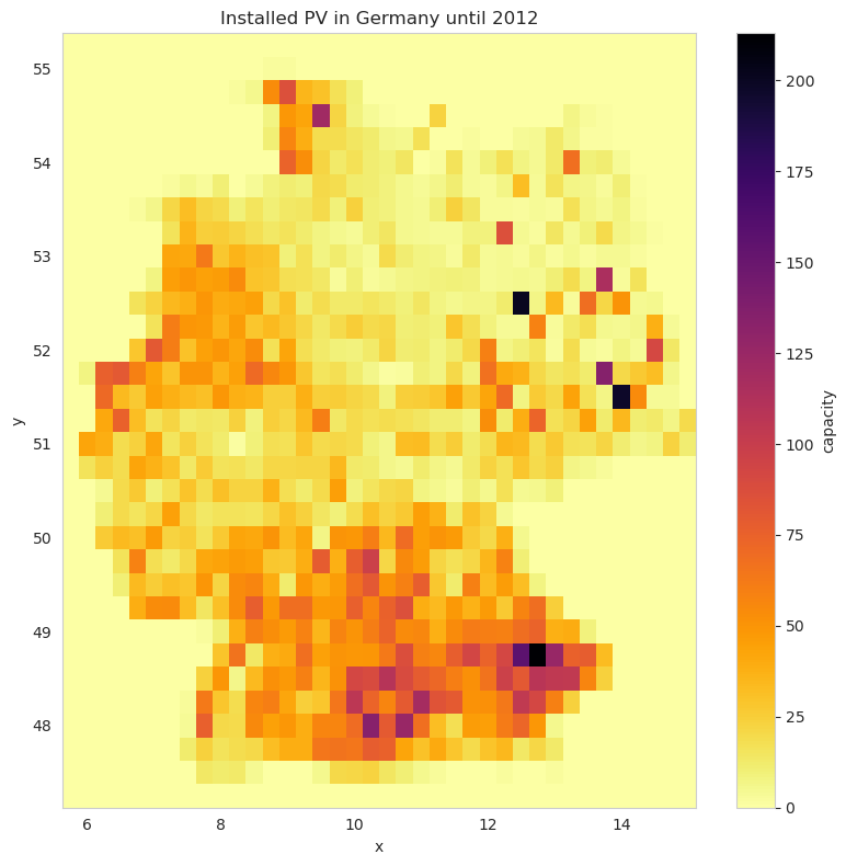
What did the total production of this capacity distribution looked like? We pass the layout to the conversion function cutout.pv. This calculates the total production over the year. We assume a south orientation ("azimuth": 180.) and prominent slope 30-35° for PV in Germany ("slope":30.)
[12]:
pv = cutout.pv(
    panel="CSi", orientation={"slope": 30.0, "azimuth": 180.0}, layout=solar_layout
)
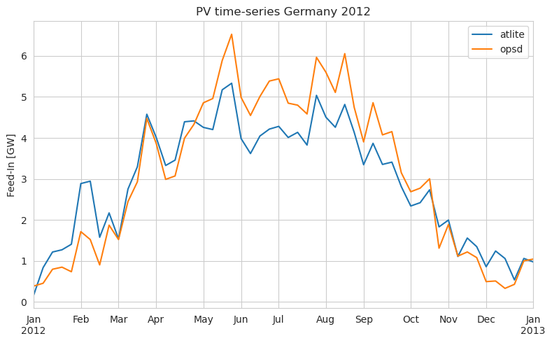
As OPSD also provides data on the total production, let’s compare those two.
[13]:
pv.squeeze().to_series()
[13]:
time
2012-01-01 00:00:00    0.0
2012-01-01 01:00:00    0.0
2012-01-01 02:00:00    0.0
2012-01-01 03:00:00    0.0
2012-01-01 04:00:00    0.0
                      ...
2012-12-31 19:00:00    0.0
2012-12-31 20:00:00    0.0
2012-12-31 21:00:00    0.0
2012-12-31 22:00:00    0.0
2012-12-31 23:00:00    0.0
Name: specific generation, Length: 8784, dtype: float64
[14]:
compare = (
    pd.DataFrame({
        "atlite": pv.squeeze().to_series(),
        "opsd": opsd["DE_solar_generation_actual"],
    })
    / 1e3
)  # in GW
compare.resample("1W").mean().plot(figsize=(8, 5))
plt.ylabel("Feed-In [GW]")
plt.title("PV time-series Germany 2012")
plt.tight_layout()
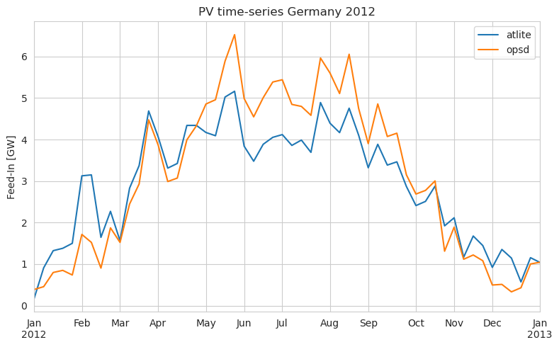
atlite also supports to set an optimal slope of the panels, using the formula documented in http://www.solarpaneltilt.com/#fixed. The production then looks like:
[15]:
pv_opt = cutout.pv(panel="CSi", orientation="latitude_optimal", layout=solar_layout)
compare_opt = (
    pd.DataFrame({
        "atlite": pv_opt.squeeze().to_series(),
        "opsd": opsd["DE_solar_generation_actual"],
    })
    / 1e3
)  # in GW
compare_opt.resample("1W").mean().plot(figsize=(8, 5))
plt.ylabel("Feed-In [GW]")
plt.title("PV time-series Germany 2012")
plt.tight_layout()
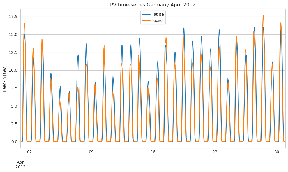
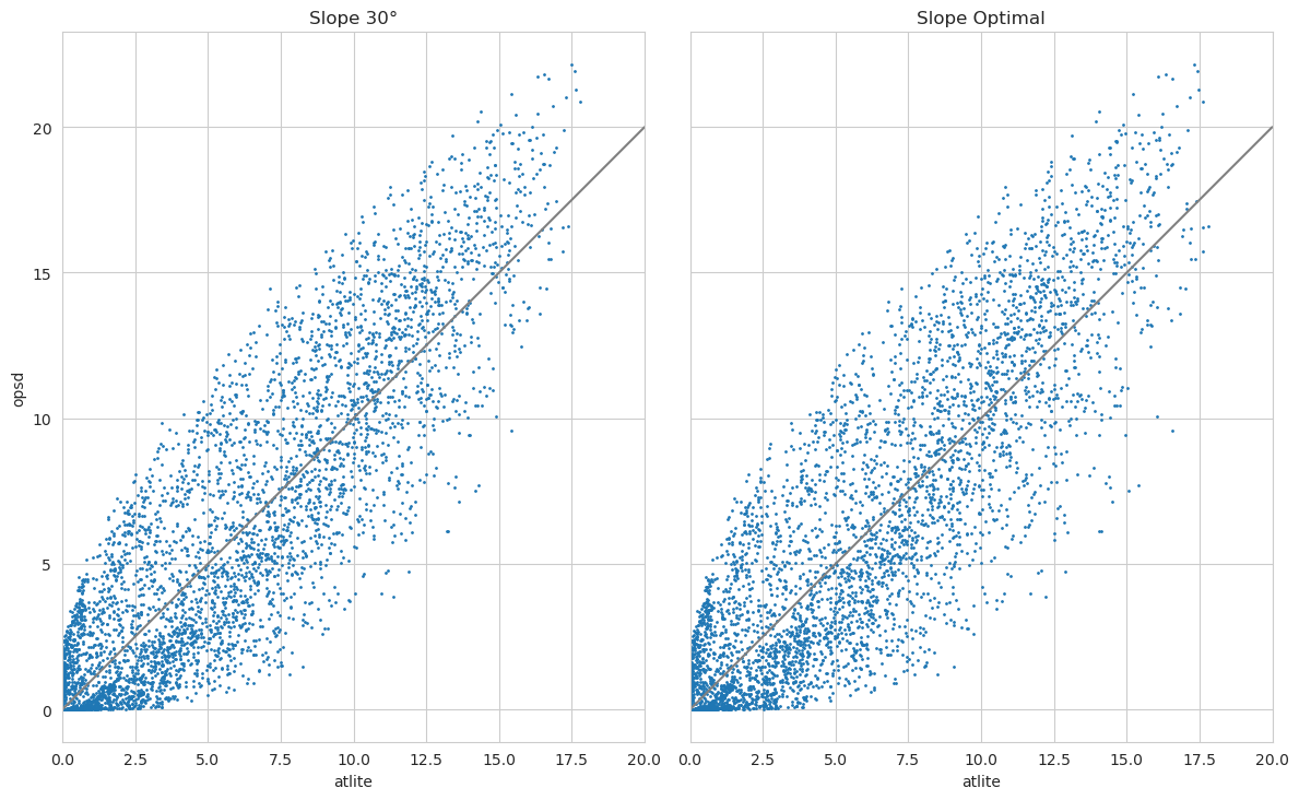
How about zooming in? Let’s plot a specific week. We see that the peaks are differing a bit. In this case atlite alternates between over and underestimating a bit… but not too bad given the fact that we are using a reanalysis dataset.
[16]:
compare_opt.loc["2012-04"].plot(figsize=(10, 6))
plt.ylabel("Feed-in [GW]")
plt.title("PV time-series Germany April 2012")
plt.tight_layout()
[17]:
fig, (ax1, ax2) = plt.subplots(
    1, 2, subplot_kw={"aspect": "equal", "xlim": [0, 20]}, figsize=(12, 16), sharey=True
)
compare.plot(x="atlite", y="opsd", kind="scatter", s=1, ax=ax1, title="Slope 30°")
compare_opt.plot(
    x="atlite", y="opsd", kind="scatter", s=1, ax=ax2, title="Slope Optimal"
)

ax1.plot([0, 20], [0, 20], c="gray")
ax2.plot([0, 20], [0, 20], c="gray")
plt.tight_layout()
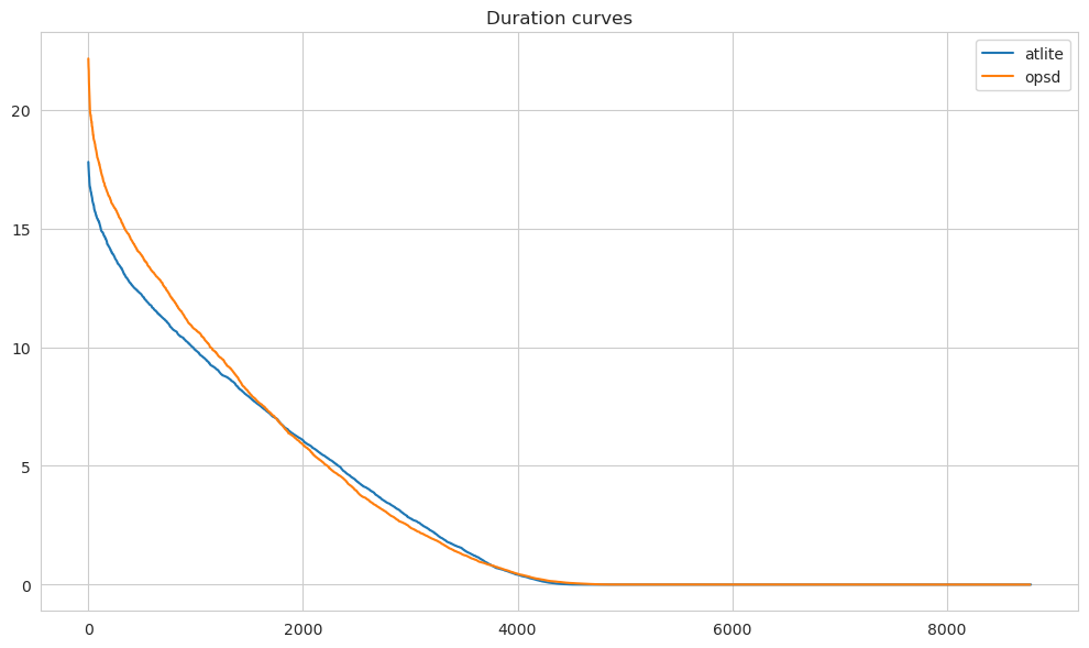
Let’s look at the duration curves of the 30° slope pv timeseries.
[18]:
compare["atlite"].sort_values(ascending=False).reset_index(drop=True).plot(
    figsize=(10, 6)
)
compare["opsd"].sort_values(ascending=False).reset_index(drop=True).plot(
    figsize=(10, 6)
)
plt.legend()
plt.title("Duration curves")
plt.tight_layout()
Examine Wind Feed-Ins#
Now we want to examine the wind potentials in Germany for year 2012.
These wind turbines are available in atlite.
[19]:
for t in atlite.windturbines:
    print(f"* {t}")
* NREL_ReferenceTurbine_2016CACost_10MW_offshore
* Vestas_V112_3MW_offshore
* NREL_ReferenceTurbine_2020ATB_7MW
* NREL_ReferenceTurbine_2019ORCost_15MW_offshore
* Vestas_V90_3MW
* Suzlon_S82_1.5_MW
* Vestas_V47_660kW
* Vestas_V25_200kW
* NREL_ReferenceTurbine_2019ORCost_12MW_offshore
* Vestas_V112_3MW
* NREL_ReferenceTurbine_2016CACost_8MW_offshore
* Enercon_E101_3000kW
* NREL_ReferenceTurbine_2020ATB_4MW
* Siemens_SWT_2300kW
* Siemens_SWT_107_3600kW
* NREL_ReferenceTurbine_2016CACost_6MW_offshore
* Bonus_B1000_1000kW
* Enercon_E82_3000kW
* NREL_ReferenceTurbine_2020ATB_18MW_offshore
* Vestas_V164_7MW_offshore
* NREL_ReferenceTurbine_2020ATB_15MW_offshore
* NREL_ReferenceTurbine_5MW_offshore
* Enercon_E126_7500kW
* Vestas_V80_2MW_gridstreamer
* NREL_ReferenceTurbine_2020ATB_5.5MW
* NREL_ReferenceTurbine_2020ATB_12MW_offshore
* Vestas_V66_1750kW
We define capacity range to roughly match the wind turbine type.
[20]:
turbine_categories = [
    {"name": "Vestas_V25_200kW", "up": 400.0},
    {"name": "Vestas_V47_660kW", "up": 700.0},
    {"name": "Bonus_B1000_1000kW", "up": 1100.0},
    {"name": "Suzlon_S82_1.5_MW", "up": 1600.0},
    {"name": "Vestas_V66_1750kW", "up": 1900.0},
    {"name": "Vestas_V80_2MW_gridstreamer", "up": 2200.0},
    {"name": "Siemens_SWT_2300kW", "up": 2500.0},
    {"name": "Vestas_V90_3MW", "up": 50000.0},
]
[21]:
low = 0
for index, turbine_cat in enumerate(turbine_categories):
    capacities = load_capacities(
        "Windkraft", cap_range=[low, turbine_cat["up"]], until="2012"
    )
    layout = cutout.layout_from_capacity_list(capacities, "capacity")

    turbine_categories[index]["layout"] = layout
    low = turbine_cat["up"]
We create a layout for each capacity range, each with a different windturbine model
[22]:
wind = xr.Dataset()
for turbine_cat in turbine_categories:
    name = f"< {turbine_cat['up']} kW"
    wind[name] = cutout.wind(
        turbine=turbine_cat["name"],
        layout=turbine_cat["layout"],
        show_progress=False,
        add_cutout_windspeed=True,
    )

wind["total"] = sum(wind[c] for c in wind)
wind
[22]:
<xarray.Dataset>
Dimensions:       (time: 8784, dim_0: 1)
Coordinates:
  * time          (time) datetime64[ns] 2012-01-01 ... 2012-12-31T23:00:00
  * dim_0         (dim_0) int64 0
Data variables:
    < 400.0 kW    (time, dim_0) float64 14.37 17.37 21.26 ... 76.24 74.27 72.48
    < 700.0 kW    (time, dim_0) float64 260.0 291.3 344.2 ... 1.276e+03 1.27e+03
    < 1100.0 kW   (time, dim_0) float64 175.9 191.8 213.9 ... 846.2 829.2 821.8
    < 1600.0 kW   (time, dim_0) float64 1.125e+03 1.208e+03 ... 4.563e+03
    < 1900.0 kW   (time, dim_0) float64 322.0 356.3 ... 1.738e+03 1.729e+03
    < 2200.0 kW   (time, dim_0) float64 991.7 1.05e+03 ... 4.803e+03 4.818e+03
    < 2500.0 kW   (time, dim_0) float64 545.8 599.2 703.2 ... 1.897e+03 1.89e+03
    < 50000.0 kW  (time, dim_0) float64 269.6 298.4 ... 1.023e+03 1.006e+03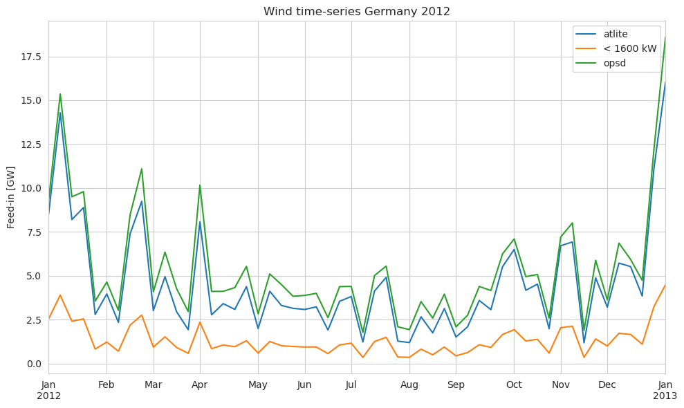
total (time, dim_0) float64 3.704e+03 4.012e+03 ... 1.617e+04Again, let’s compare the result with the feed-in statistics from OPSD. We add an extra column for wind turbines with capacity lower than 1600 kW
[23]:
compare = pd.DataFrame({
    "atlite": wind["total"].squeeze().to_series(),
    "< 1600 kW": wind["< 1600.0 kW"].squeeze().to_series(),
    "opsd": opsd["DE_wind_generation_actual"],
})

compare = compare / 1e3  # in GW
[24]:
compare.resample("1W").mean().plot(figsize=(10, 6))
plt.ylabel("Feed-in [GW]")
plt.title("Wind time-series Germany 2012")
plt.tight_layout()
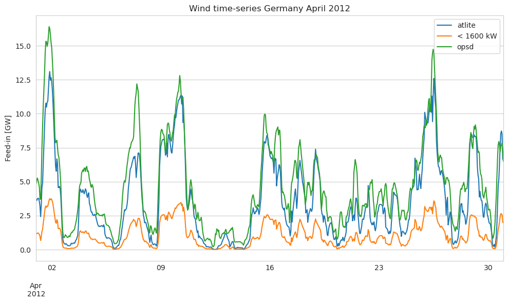
[25]:
compare.loc["2012-04"].plot(figsize=(10, 6))
plt.ylabel("Feed-in [GW]")
plt.title("Wind time-series Germany April 2012")
plt.tight_layout()
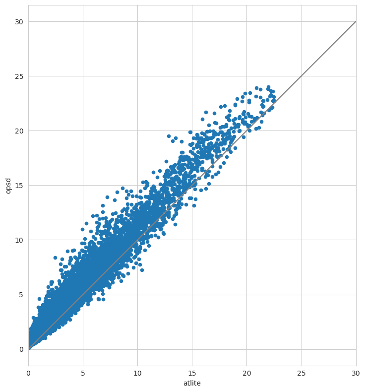
[26]:
ax = compare.plot(x="atlite", y="opsd", kind="scatter", figsize=(12, 8))
ax.set_aspect("equal")
ax.set_xlim(0, 30)
ax.plot([0, 30], [0, 30], c="gray")
plt.tight_layout()
[27]:
compare["atlite"].sort_values(ascending=False).reset_index(drop=True).plot(
    figsize=(10, 6)
)
compare["opsd"].sort_values(ascending=False).reset_index(drop=True).plot(
    figsize=(10, 6)
)
plt.legend()
plt.title("Duration curves")
plt.ylabel("Wind Feed-in [GW]")
plt.xlabel("Accumulated hours")
plt.tight_layout()
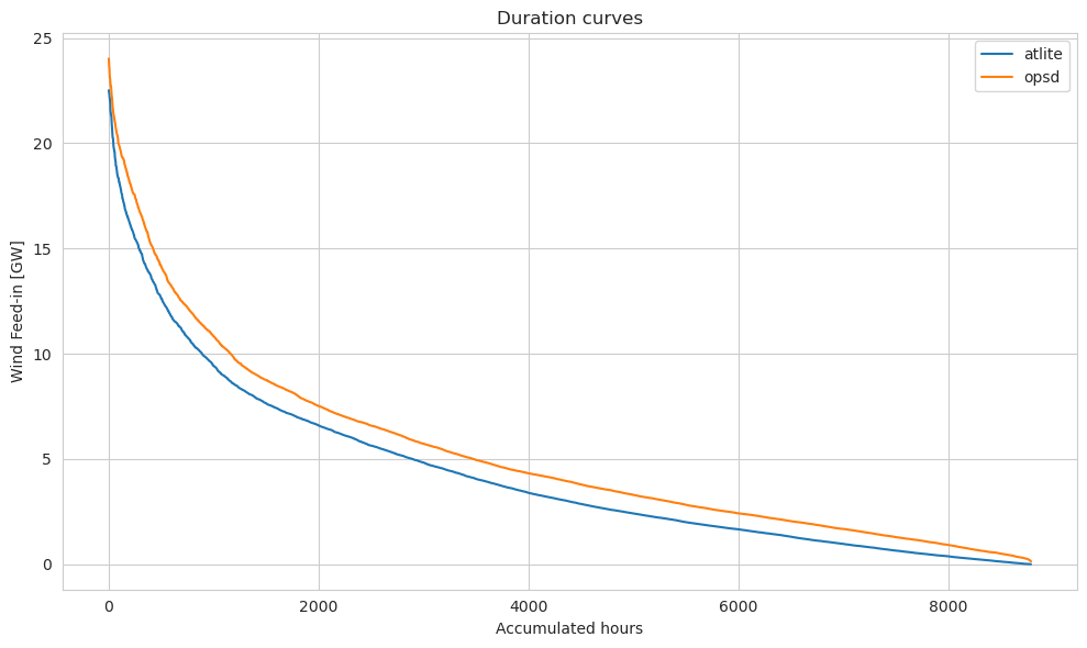
Looks quite aggreeable!
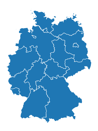
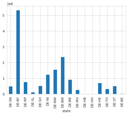
Splitting time-series into shapes#
The generation time-series can also be aggregated based on shapes. In this example, we aggregate on the basis of the German “Länder” (federal states).
[28]:
shp = shpreader.Reader(
    shpreader.natural_earth(
        resolution="10m", category="cultural", name="admin_1_states_provinces"
    )
)
de_records = list(
    filter(lambda r: r.attributes["iso_3166_2"].startswith("DE"), shp.records())
)
laender = (
    gpd
    .GeoDataFrame([{**r.attributes, "geometry": r.geometry} for r in de_records])
    .rename(columns={"iso_3166_2": "state"})
    .set_index("state")
    .set_crs(4236)
)
[29]:
laender.to_crs(3035).plot(figsize=(7, 7))
plt.grid(False)
plt.axis("off");
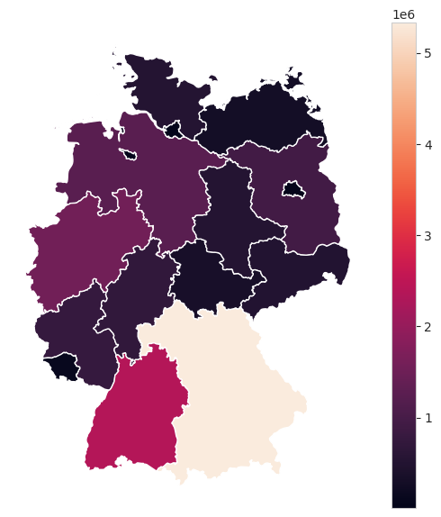
[30]:
pv = cutout.pv(
    panel="CSi",
    orientation={"slope": 30.0, "azimuth": 0.0},
    shapes=laender,
    layout=solar_layout,
)
[31]:
production = pv.sum("time").to_series()
laender.plot(column=production, figsize=(7, 7), legend=True)
plt.grid(False)
plt.axis("off");
/home/fabian/.miniconda3/lib/python3.11/site-packages/geopandas/plotting.py:732: FutureWarning: is_categorical_dtype is deprecated and will be removed in a future version. Use isinstance(dtype, CategoricalDtype) instead
  if pd.api.types.is_categorical_dtype(values.dtype):
[32]:
production.plot(kind="bar");
[ ]: